I. Metaballs
I will begin with a brief review of what a metaball is, for newbies. A metaball is an isosurface in 3D space. Basically, define a function in 3D space, which takes as input the x,y,z coordinates of a point, and outputs a floating point value. Then decide on a threshold for this output; points in 3D space that fall below the threshold (when run through the function) are ONE, while points above the threshold are ZERO. This divides 3D space into two sets - think of it as solid (occupied) space versus empty space (air). The continuous surface that is formed where the two meet (assuming the function's output is continuous/differentiable) is called an isosurface. This isosurface has a different look for each possible function. The function [f(x,y,z) = x^2 + y^2 + z^2] will have a value of zero at the origin, and for any other point, its value will be the distance from the origin. Therefore the isosurface created by this function (when you take the output vs. a threshold value) will create a beautiful, perfect sphere. (The radius of the sphere is the square root of the threshold.) However, we've all seen spheres a million times in raytracing, and they get kind of boring, right? Another possible function: [f(x,y,z) = ax + by + cz]. This will divide space in half along a plane, whose normal is
Next, I show you where the point charges lie that create the electric field, marked by nice purple dots. They are of varying strengths:
Now, I'm sure you've seen a topography map before, where bands of color are equated to certain discrete heights in terrain. Here, we do the same thing, but we map the electric field strength into several discrete color bands. Think of it as a height map in a natural park. Here are 6 bands, and 9 bands, respectively:

Above, where you see a contour, this is an equipotential line - a line along which the potential (physics jargon for the electric field strength) is equal at all points. Now, think about what would happen to our 'terrain map' if there was a great flood. This would divide it into two parts - one above the water, and one below. The shoreline would be an equipotential line, right? Okay, so now bring yourself back to the 2D (flat image) realm. Say we pick some threshold value at which to place an equipotential line, like the white one in this image:
Next we divide space along this line. We want to categorize every point in space, based on whether or not it's inside, or outside, of some arbitrary shape, or whether or not the electric field strength exceeds the threshold there. We get this:

Nice blobs, yes? Now, picture doing this in 3D space instead of 2D space. When you draw these equipotential lines, they actually become equipotential surfaces, otherwise known as isosurfaces, as we were talking about before. And they form beautiful, 3-dimensional blobs...
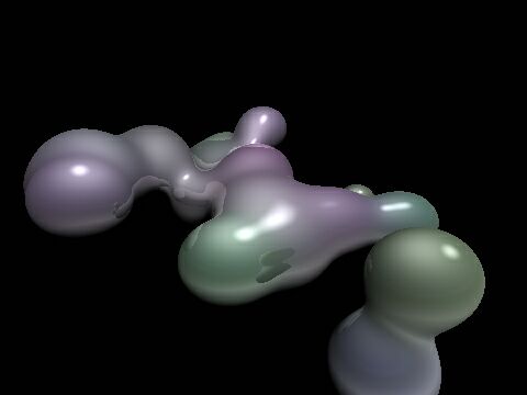
II. Rendering
Now, rendering a sphere is easy. You cast a ray from the camera's point in 3D space through a pixel in a 2D grid of pixels (the screen), and you solve, mathematically, for the intersection of the sphere and the ray. There are either 0, 1, or 2 solutions (the quadratic equation is used), corresponding to the distances to intersection. If you have multiple spheres in the scene, you test the ray for intersection with each sphere, then take the lowest number (the closest sphere), you determine its color there (dot the sphere normal with the vector to the light source, etc.), plot the color, and move on to the next pixel. However, rendering blobs is not so easy. Say you have 50 point charges. We could consider 50 spheres all separately - for each, we just solve a quadratic equation. However, with 50 point charges, we're going to be solving some kind of 50th-degree polynomial. And that's not easy. =) So what do we do? We cheat. We're going to 'inch' along a ray cast from the camera in the direction of the pixel. At each point in 3D space, we evaluate the 3D blob function (a sum of 50 blob functions, based on the x/y/z coordinates of that point, and the coordinates of each point charge). When (if) we finally find a point along that ray that is above our threshold, voila - we've hit the blob. We determine color information, plot it, and move on to the next pixel. However, this is a very slow process. It seems inevitable that we have to inch along the ray in tiny increments to avoid a 'jittery' image. (Some optimizations can be made for this - they will be discussed later.) However, at every point along that ray, we have to calculate the blob function for all 50 charges. Also notice that each involves 3 floating- point multiplies, two adds, and a divide. That spells S-L-O-W, and the divide is the culprit. How to make it faster? Well. Hmmm. Here's my little discovery. It could be something lots of other people have figured out, and in fact probably is, but I did develop it on my own. And now I share it with you.III. An Optimization
We replace the equation 1/r^2 with the equation [g(r) = r^4 - r^2 + 0.25]. See the graphs below. Notice that it has the convenient property that at g(0) = 0.25 (which actually handles better than +infinity), and g(0.707) = 0; so at a distance of sqrt(2)/2 (or 0.707) from the charge, there is no electric field contribution. Additionally, the values between r=0 and r=0.707 smoothly range from 0.25 down to 0, but they do so in a nonlinear fashion, which is the property of the 1/r^2 equation that creates the 'blobbiness' of the summed fields. For now, assume that the value of g beyond g(0.707) is just zero. (In the code we'll just set q to zero when r > 0.707).
Now, a lot of good this does, right? Right! Here's the trick: the electric field contribution due to a charge no longer reaches to infinity! It dies off completely at a distance of 0.707 from the charge (if you ignore points where r > 0.707). This means that each charge has a limited sphere of influence, which we will hereafter call its bounding sphere. So, as we inch along the ray, we only have to add the electric field contributions from the point charges for which the current point on the ray is inside the bounding sphere. This is often a very, very small fraction of the whole population of charges in the scene, and rendering time plummets. ** Update ** (March 2011 - long overdue - my apologies) Ken Perlin came up with another nice basis function that works well for this purpose. The equation (graphed below) is: g(r) = 6r^5 - 15r^4 + 10r^3 ...or... g(r) = r * r * r * (r * (r * 6 - 15) + 10) One nice thing about this is that the range of r is from [0..1], rather than [0..0.707]. The other nice thing is that it's actually symmetrical about the midpoint, with zero-derivatives at both g(0) and g(1) - so you can use it for a kind of general "smoothing" function, for all kinds of purposes, even outside of graphics. Note that this curve is inverted from the curve we use for blobs; here, g(0) = 0, and g(1) = 1. With blobs, we want g(0) ~= 1, and g(1) ~= 0. Because of this equation's symmetry, you can invert either the domain or the range, and it will work (i.e. take g(1-r), or take 1-g(r)).
 The blue line is simply g(r) = r, while the red line is the 'smoothed'
version, g(r) = 6r^5 - 15r^4 + 10r^3. For the latter, note the nice
zero-slope at both r==0 and r==1, and the symmetry about the center.
(now back to our main lesson...)
Here's how it works, in pseudocode:
For each pixel, cast a ray out
Determine the intersection of the ray with all point charges' bounding spheres
Sort the intersections (both entries & exits!)
For each intersection (from nearest to farthest)
If 'entry' (into bounding sphere): add that charge to 'active' list;
Else ('exit' from bounding sphere): remove that charge from 'active' list.
Now trace along the ray from this intersection to the next intersection,
using the 'active' list as the point charges contributing to the field.
The 'active' list is just a list of the charges (it starts empty) that are currently
contributing. As we move along the ray and enter the sphere of influence of certain
charges, they get added to the list. As we exit the spheres of influence of charges, they
are removed from the list. For optimal performance, we calculate all the ray's
intersections with the bounding spheres at the start, sort them, and inch along the ray,
only interrupting to modify the 'active' list when we cross (enter or exit) a bounding
sphere.
So, this way, we can have a million charges in our scene, and still, only the ones that fall
very close to a ray from the camera will actually get considered in the electric field
summation. All million charges are, however, considered in the bounding sphere
calculation (most will yield 0 intersections though), and we have to sort the successful
intersections, but this sorting is negligible in comparison. (Note that a merge sort is
probably best here.) From my experience, doing all this is well worth the effort - and the
more charges you have, the more this algorithm benefits next to the original,
exponentially. With a complicated scene (2000 charges), it renders a scene from 20 to 50
times faster!
Here is an example image - the same one as before - but it shows, in red, the area that is
outside the bounding spheres:
The blue line is simply g(r) = r, while the red line is the 'smoothed'
version, g(r) = 6r^5 - 15r^4 + 10r^3. For the latter, note the nice
zero-slope at both r==0 and r==1, and the symmetry about the center.
(now back to our main lesson...)
Here's how it works, in pseudocode:
For each pixel, cast a ray out
Determine the intersection of the ray with all point charges' bounding spheres
Sort the intersections (both entries & exits!)
For each intersection (from nearest to farthest)
If 'entry' (into bounding sphere): add that charge to 'active' list;
Else ('exit' from bounding sphere): remove that charge from 'active' list.
Now trace along the ray from this intersection to the next intersection,
using the 'active' list as the point charges contributing to the field.
The 'active' list is just a list of the charges (it starts empty) that are currently
contributing. As we move along the ray and enter the sphere of influence of certain
charges, they get added to the list. As we exit the spheres of influence of charges, they
are removed from the list. For optimal performance, we calculate all the ray's
intersections with the bounding spheres at the start, sort them, and inch along the ray,
only interrupting to modify the 'active' list when we cross (enter or exit) a bounding
sphere.
So, this way, we can have a million charges in our scene, and still, only the ones that fall
very close to a ray from the camera will actually get considered in the electric field
summation. All million charges are, however, considered in the bounding sphere
calculation (most will yield 0 intersections though), and we have to sort the successful
intersections, but this sorting is negligible in comparison. (Note that a merge sort is
probably best here.) From my experience, doing all this is well worth the effort - and the
more charges you have, the more this algorithm benefits next to the original,
exponentially. With a complicated scene (2000 charges), it renders a scene from 20 to 50
times faster!
Here is an example image - the same one as before - but it shows, in red, the area that is
outside the bounding spheres:
IV. Control
Many factors allow you to control the look of the blobs. One is the strength of the charge, which will determine how big that 'chunk' of the blob is. This is just a number that scales the contribution of the charge to the net electric field. You can also adjust the threshold. Remember, its function is to decide what is blob vs. what is open space. If the net electric field somewhere is greater than the threshold, then that point is inside (or on the surface of) the blob volume. Valid threshold ranges are from 0.0 to 0.25. At 0.0001, you will have blobs that basically look like spheres, and they will take up the entire volume of the bounding spheres. At 0.24, you will get very small blobs that take up a tiny percentage of the bounding spheres - not very useful. A medium value of 0.15 to 0.2 seems to work best, giving you optimal use of the bounding spheres, and a good 'blobbing-together' look. You can also implement other shapes, such as the cube, the torus (donut), and others. I leave this to you to figure out, though. Here are some cubes: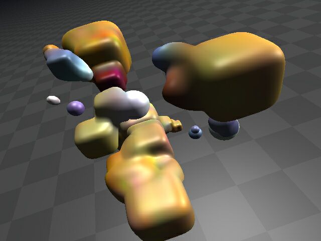
And the classic donut:
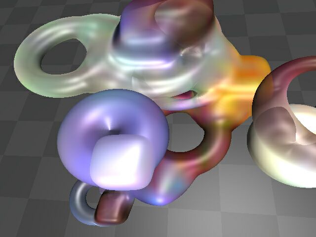
V. Miscellaneous
A note about normals. If you're smart, you can figure this one out. Say you're inching along a ray in 3D space and all of a sudden you hit the blob. What's the next thing you do? You try to figure out what color to plot. You have the 3D coordinates of the ray- blob intersection. But you want realistic lighting, so you have to get the normal (a vector perpendicular to the blob surface) at that point. You can then dot this normal with a vector to the light source(s) and figure out the appropriate lighting. How to get this normal? Pretend your point charges are just spheres. Get the normal of each sphere, as a unit vector, pretending that the point lies on the sphere. (All this involves is subtracting two points in space and normalizing the vector to unit length - do this once for each point charge.) So now you have a bunch of normals. How do you 'blend' them together to get the real normal? Just do a weighted average. You know the net electric field value at this point, call it 'q' (and it's obviously at or slightly above the threshold value). Just look at the electric field contribution of each point charge, q(i). They all add up to 'q'. So just use these as the weights to your normals, do a linear combination (add up the normals weighted by the q(i)'s), divide by the total weight, q, and voila, you have the normal. Note that you can also assign each point charge its own color, transparency value, refraction value, shininess, texture strength(s), reflectivity, etc. You can then use the normal interpolation technique in the same way (only, you're just doing a linear combination of scalars, not vectors, this time) to smoothly vary the surface characteristics of the blob. For instance, you can vary the color of the different "globs" in the blob shape (you can find examples of this throughout this document). You could also have some parts of the blob be transparent while others are solid and highly reflective. There are infinite possibilities. Also, be sure to experiment with things like reflection and refraction, and procedural textures in 3D space are very cool. You can base them on either the point in 3D space or on the normal itself (this can be very interesting). This one (below) is just a normal perturbation based on a high-frequency sine function of the sum of the x, y, and z coordinates. Notice the nice shiny highlights on the bumps - one of the advantages of perturbing the normal: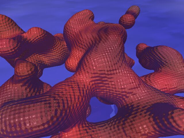
Well, that brings this educational FAQ to an end. I hope you've enjoyed the pictures and maybe even learned something. On a final note, we should all cut back a bit on the amount of meat we eat so that fewer billions of animals are slaughtered each year. Personally, I'd have trouble making the vegetarian transition; but I think eating less meat is important. Thanks for listening! UPDATE, 5/24/01: I lied; I made the vegetarian transition about a month ago; it was easy, and I feel great about it. Read all about it on the what's new page (if it's still there).
VI. BONUS UPDATES (5/24/01)
I just went digging into some of my old blobs code and found the equations I came up with for doing cubes & torii, for which I've had several requests in the past, so here they are. I haven't beautified it at all; you have to be able to decipher my cryptic "notes to self" to win the reward on this one... =) btw, a tip: 'mag' is the magnitude of the current charge (blob node) under consideration.
SPHERES
-----------------------
isometric surface equation: x^2 + y^2 + z^2 = mag^2
radius = mag
radius (mag) represents largest possible area of contribution
-> the spherical bounding test uses the radius (squared).
CUBES
-----------------------
isometric surface equation: x^4 + y^4 + z^4 = mag^4
max radius = sqrt(sqrt(2.0))*mag [corners]
min raduis = mag [flat edges]
mag (min radius) represents 1/2 the length of a cube edge
isometric volume represents largest possible area of contribution
-> the spherical bounding test uses the max radius (squared).
-> the bounding box test uses the min radius as the distance of the
planes from the "origin."
TORII
-----------------------
basically, there's an "axis ring" whose radius is 'mag'.
the largest possible area of contribution is a torus around that axis, of sub-radius
'inner_rad'.
isometric surface equation: [closest dist. to axis ring]^2 = inner_rad^2
-> 'inner' radius can be greater than 'mag' (makes apples w/dimples), but it must not
be more than 2x as big as it (untested circumstance).
-> math note: the "closest distance" is a 3D function broken down into fake 2D:
it gets the distance to it in y, and in x/z, then does a 2D distance on those. Slick!
-> the spherical bounding test uses the radius 'mag + inner_rad'.
-> this is followed by a clip at y=inner_rad and y=-inner_rad.
-> this is follwed by a complicated test:
[rc (radius of cylinder) = mag - inner_rad]
if the entry point of the ray was cut off on a y-plane and that cut-off entry
point is inside the cylinder x^2 + z^2 = rc^2, then start the span at the far
end of the cylinder.
...and here's some (unoptimized for legibility) sample code:
if (blob[k].type == C_SPHERE)
{
dx = (p.x - blob[k].x);
dy = (p.y - blob[k].y);
dz = (p.z - blob[k].z);
r_squared = (dx*dx + dy*dy + dz*dz);
//enable this line if your blobs are of varying sizes:
//r_squared /= (blob[k].mag*blob[k].mag);
// since f(r) is valid when r is in the range [0-.707],
// r_squared should be in the range [0-.500].
if (r_squared < 0.5f) // same as: if (sqrtf(r_squared) < 0.707f)
{
q += (0.25 - r_squared + r_squared*r_squared);
}
}
else if (blob[k].type == C_CUBE)
{
dx = p.x - blob[k].x;
dy = p.y - blob[k].y;
dz = p.z - blob[k].z;
dx *= dx;
dy *= dy;
dz *= dz;
dx *= dx;
dy *= dy;
dz *= dz;
r_4th = dx + dy + dz;
if (r_4th <= blob[k].mag_4th) // r < 0.7*blob[k].mag đ r^2 < 0.5*blob[k].mag
{
r_4th *= blob[k].half_mag_inv_4th;
q += (0.25 - r_4th + r_4th*r_4th);
}
}
else if (blob[k].type == C_TORUS)
{
float dist_in_xz, dist_in_y, dist_from_track_squared;
dx = p.x - blob[k].x;
dy = p.y - blob[k].y;
dz = p.z - blob[k].z;
dist_in_xz = sqrt(dx*dx + dz*dz) - blob[k].mag;
dist_in_y = dy;
dist_from_track_squared = (dist_in_xz*dist_in_xz + dist_in_y*dist_in_y);
if (dist_from_track_squared < blob[k].inner_rad*blob[k].inner_rad)
{
dist_from_track_squared *= 0.5/(blob[k].inner_rad*blob[k].inner_rad);
q += (0.25 - dist_from_track_squared + dist_from_track_squared*dist_from_track_squared);
}
}
OTHER TIPS:
* For fast tessellation using marching cubes, consider a surface-crawler. (This is what I used for Geoforms.)
* For fast splatting, consider using an octree. (This is what I used for Lava aka Oozic.)
Back to Top
Back to Raytracing
This document and all images are copyright (c)2000+ Ryan Geiss.
Please maintain credit to author upon citation or duplication.